Spherical Harmonic Models 2
# Import notebook dependencies

import sys
sys.path.append('..')
import matplotlib.pyplot as plt
plt.style.use('seaborn-white')
import numpy as np
import pandas as pd
from src import sha_lib as sha
import os
1. A more tangible example of modelling using spherical harmonics
First, there’s a data file with some spatial data to plot.
# Load the data
lsfile = '../data/external/land_5deg.csv'
lsdata = np.genfromtxt(lsfile, delimiter=',')

x = lsdata[:,0].reshape(36, 72)
y = lsdata[:,1].reshape(36,72)
z = lsdata[:,2].reshape(36,72)

# Plot them
plt.rcParams['figure.figsize'] = [15, 8]
plt.contourf(x,y,z)
plt.colorbar()
plt.show()
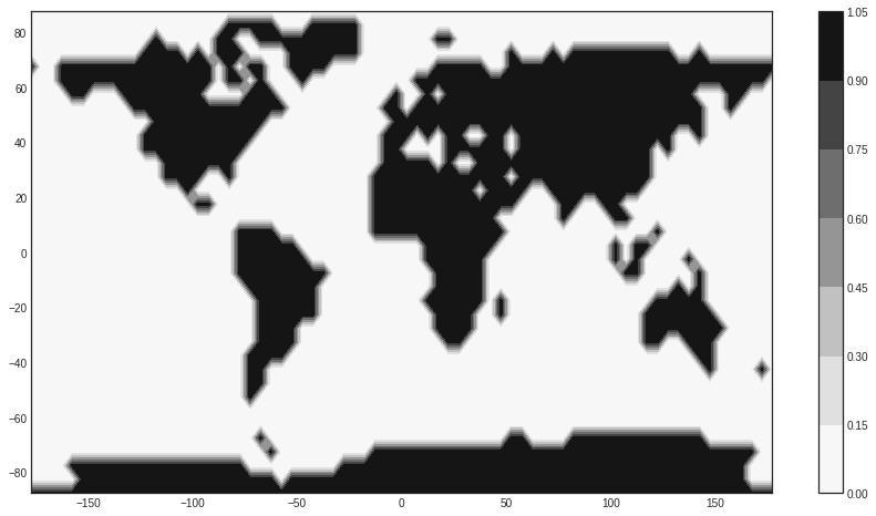
The data file consists of binary values (1=land, 0=water) on a 5-degree grid. We now take these data as the input to a global spherical harmonic analysis and calculate a spherical harmonic model with a user specified resolution.
>> USER INPUT HERE: Set the maximum spherical harmonic degree of the analysis
nmax = 5 # Max degree
# These functions are used for the spherical harmonic analysis and synthesis steps
# Firstly compute a spherical harmonic model of degree and order nmax using the input data as plotted above
def sh_analysis(lsdata, nmax):
    npar = (nmax+1)*(nmax+1)
    ndat = len(lsdata)
    lhs  = np.zeros(npar*ndat).reshape(ndat,npar)

    rhs  = np.zeros(ndat)
    line = np.zeros(npar)
    ic   = -1
    for i in range(ndat):
        th  = 90 - lsdata[i][1]
        ph  = lsdata[i][0]
        rhs[i] = lsdata[i][2]
        cmphi, smphi = sha.csmphi(nmax,ph)
        pnm = sha.pnm_calc(nmax, th)
        for n in range(nmax+1):
            igx = sha.gnmindex(n,0)
            ipx = sha.pnmindex(n,0)
            line[igx] = pnm[ipx]
            for m in range(1,n+1):
                igx = sha.gnmindex(n,m)
                ihx = sha.hnmindex(n,m)
                ipx = sha.pnmindex(n,m)
                line[igx] = pnm[ipx]*cmphi[m]
                line[ihx] = pnm[ipx]*smphi[m]
        lhs[i,:] = line

    shmod  = np.linalg.lstsq(lhs, rhs.reshape(len(lsdata),1), rcond=None)
    return(shmod)


# Now use the model to synthesise values on a 5 degree grid in latitude and longitude
def sh_synthesis(shcofs, nmax):
    newdata =np.zeros(72*36*3).reshape(2592,3)
    ic = 0
    for ilat in range(36):
        delta = 5*ilat+2.5
        lat = 90 - delta
        for iclt in range(72):
            corr  = 5*iclt+2.5
            long  = -180+corr
            colat = 90-lat
            cmphi, smphi = sha.csmphi(nmax,long)
            vals  = np.dot(sha.gh_phi(shcofs, nmax, cmphi, smphi), sha.pnm_calc(nmax, colat))
            newdata[ic,0]=long
            newdata[ic,1]=lat
            newdata[ic,2]=vals
            ic += 1
    return(newdata)
# Obtain the spherical harmonic coefficients
shmod = sh_analysis(lsdata=lsdata, nmax=nmax)
# Read the model coefficients
shcofs = shmod[0]
# Synthesise the model coefficients on a 5 degree grid
newdata = sh_synthesis(shcofs=shcofs, nmax=nmax)
# Reshape for plotting purposes
x = newdata[:,0].reshape(36, 72)
y = newdata[:,1].reshape(36,72)
z = newdata[:,2].reshape(36,72)
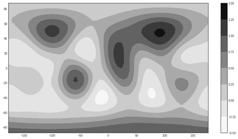
# Plot the results
plt.rcParams['figure.figsize'] = [15, 8]
levels = [-1.5, -0.75, 0, 0.25, 0.5, 0.75, 2.]
plt.contourf(x,y,z)
plt.colorbar()
plt.show()
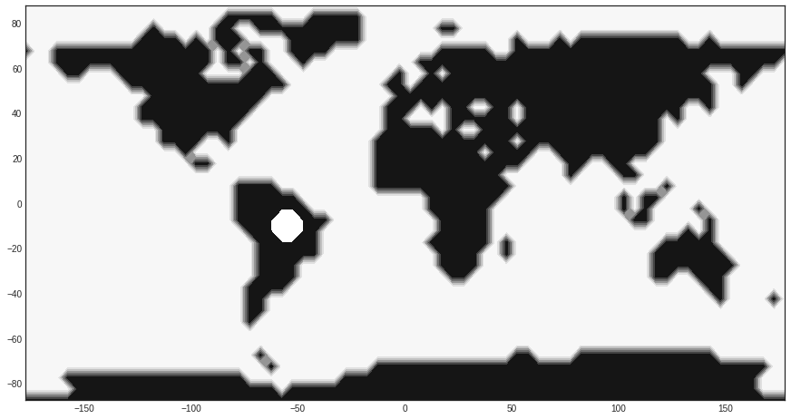
Spherical harmonic models with data gaps
What happens if the data set is incomplete? In this section, you can experiment by removing data within a great circle of a specified radius and position. The functions below are used to create the data gap, and the modelling uses functions in the above section again.
def greatcircle(th1, ph1, th2, ph2):
    th1 = np.deg2rad(th1)
    th2 = np.deg2rad(th2)
    dph = np.deg2rad(dlong(ph1,ph2))

  # Apply the cosine rule of spherical trigonometry
    dth = np.arccos(np.cos(th1)*np.cos(th2) + \
              np.sin(th1)*np.sin(th2)*np.cos(dph))
    return(dth)

def dlong (ph1, ph2):
    ph1 = np.sign(ph1)*abs(ph1)%360   # These lines return a number in the
    ph2 = np.sign(ph2)*abs(ph2)%360   # range -360 to 360
    if(ph1 < 0): ph1 = ph1 + 360      # Put the results in the range 0-360
    if(ph2 < 0): ph2 = ph2 + 360
    dph = max(ph1,ph2) - min(ph1,ph2) # So the answer is positive and in the
                                      # range 0-360
    if(dph > 180): dph = 360-dph      # So the 'short route' is returned
    return(dph)

def gh_phi(gh, nmax, cp, sp):
    rx = np.zeros(nmax*(nmax+3)//2+1)
    igx=-1
    igh=-1
    for i in range(nmax+1):
        igx += 1
        igh += 1
        rx[igx]= gh[igh]
        for j in range(1,i+1):
            igh += 2
            igx += 1
            rx[igx] = (gh[igh-1]*cp[j] + gh[igh]*sp[j])
    return(rx)
>> USER INPUT HERE: Set the location and size of the data gap
Colatitude: degrees
Longitude: degrees
Radius: km
# Remove a section of data centered on colat0, long0 and radius here
colat0 = 100
long0  = -55
radius  = 500
lsdata_gap = lsdata.copy()
for row in range(len(lsdata_gap)):
    colat = 90 - lsdata_gap[row,1]
    long  = lsdata_gap[row,0]
    if greatcircle(colat, long, colat0, long0) < radius/6371.2:
        lsdata_gap[row,2] = np.nan

print('Blanked out: ', np.count_nonzero(np.isnan(lsdata_gap)))

x_gap = lsdata_gap[:,0].reshape(36, 72)
y_gap = lsdata_gap[:,1].reshape(36,72)
z_gap = lsdata_gap[:,2].reshape(36,72)

# Plot the map with omitted data
plt.contourf(x_gap, y_gap, z_gap)
Blanked out: 4
<matplotlib.contour.QuadContourSet at 0x7fdd73b5f9d0>
>> USER INPUT HERE: Set the maximum spherical harmonic degree of the analysis
nmax = 5 #Max degree
# Select the non-nan data
lsdata_gap = lsdata_gap[~np.isnan(lsdata_gap[:,2])]

# Obtain the spherical harmonic coefficients for the incomplete data set
shmod = sh_analysis(lsdata=lsdata_gap, nmax=nmax)

# Read the model coefficients
shcofs = shmod[0]

# Synthesise the model coefficients on a 5 degree grid
newdata = sh_synthesis(shcofs=shcofs, nmax=nmax)
# Reshape for plotting purposes
x_new = newdata[:,0].reshape(36, 72)
y_new = newdata[:,1].reshape(36,72)
z_new = newdata[:,2].reshape(36,72)
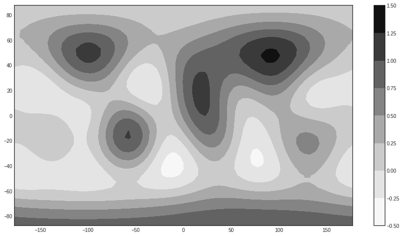
Print the maximum and minimum of the synthesised data. How do they compare to the original data, which was composed of only ones and zeroes? How do the max/min change as you vary the data gap size and the analysis resolution? Try this with a large gap, e.g. 5000 km.
print(np.min(z_new))
print(np.max(z_new))
-0.34396515044758263
1.2946196188811945
# Plot the results with colour scale according to the data
plt.rcParams['figure.figsize'] = [15, 8]
plt.contourf(x_new, y_new, z_new)
plt.colorbar()
plt.show()
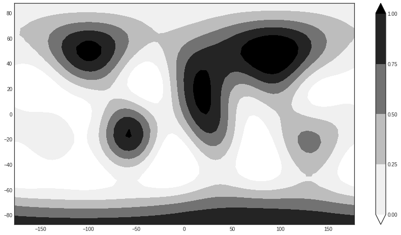
Now see what happens when we restrict the colour scale to values between 0 and 1 regardless of the data values (so that both ends of the colour scale are saturated).
# Plot the results
plt.rcParams['figure.figsize'] = [15, 8]
levels = [0, 0.25, 0.5, 0.75, 1.]
plt.contourf(x_new, y_new, z_new, levels, extend='both')
plt.colorbar()
plt.show()
Making a spherical harmonic model of the geomagnetic field
There is a file containing virtual observatory (VO) data calculated from the Swarm 3-satellite constellation in this repository. VOs use a local method to provide point estimates of the magnetic field at a specified time and fixed location at satellite altitude. This technique has various benefits, including:
Easier comparison between satellite (moving instrument) and ground observatory (fixed instrument) data, which is particularly useful when studying time changes of the magnetic field, e.g. geomagnetic jerks.
One can compute VOs on a regular spatial grid to mitigate the effects of uneven ground observatory coverage.
A brief summary of the method used to calculate each of these VO data points:
Swarm track data over four months are divided into 300 globally distributed equal area bins
Gross outliers (deviating over 500nT from the CHAOS-6-x7 internal field model) are removed
Only data from magnetically quiet, dark times are kept
Estimates of the core and crustal fields from CHAOS-6-x7 are subtracted from each datum to give the residuals
A local magnetic potential \(V\) is fit to the residuals within the cylinder
Values of the residual magnetic field in spherical coordinates (\(r\), \(\theta\), \(\phi\)) are computed from the obtained magnetic potential using \(B=-\nabla V\) at centre of the bin (at 490km altitude)
An estimate of the modelled core field at the VO calculation point is added back onto the residual field to give the total internal magnetic field value
In this section, we will use VOs as input data for a degree 13 spherical harmonic model of the geomagnetic field at 2015.0 and compare our (satellite data only) model to the latest IGRF (computed using both ground and satellite data) at the same time.
# Read in the VO data
cfile = '../data/external/SwarmVO_IAGASummerSchool.dat'
cols  = ['Year','Colat','Long','Rad','Br','Bt', 'Bp']
bvals = pd.read_csv(cfile, sep='\s+', skiprows=0, header=None, index_col=0,
                    na_values=[99999.00,99999.00000], names=cols, comment='%')
bvals = bvals.dropna()
bvals['Bt']= -bvals['Bt']
bvals['Br']= -bvals['Br']
colnames=['Colat','Long','Rad','Bt','Bp', 'Br']
bvals=bvals.reindex(columns=colnames)
bvals.columns = ['Colat','Long','Rad','X','Y','Z']

# Set the date to 2015.0 (this is the only common date between the VO data file and the IGRF coefficients file)
epoch = 2015.0
# Set the model resolution to 13 (the same as IGRF)
nmax = 13
def geomagnetic_model(epoch, nmax, data, RREF=6371.2):
    # Select the data for that date
    colat =  np.array(data.loc[epoch]['Colat'])
    nx   = len(colat) # Number of data triples
    ndat = 3*nx    # Total number of data
    elong =  np.array(data.loc[epoch]['Long'])
    rad   =  np.array(data.loc[epoch]['Rad'])
    rhs   =  data.loc[epoch][['X', 'Y', 'Z']].values.reshape(ndat,1)
    npar = (nmax+1)*(nmax+1) # Number of model parameters
    nx   = len(colat) # Number of data triples
    ndat = 3*nx    # Total number of data

    # Arrays for the equations of condition
    lhs  = np.zeros(npar*ndat).reshape(ndat,npar)
    linex = np.zeros(npar); liney = np.zeros(npar); linez = np.zeros(npar)

    iln = 0 # Row counter
    for i in range(nx): # Loop over data triplets (X, Y, Z)
        r  = rad[i]
        th = colat[i]; ph  = elong[i]
        rpow = sha.rad_powers(nmax, RREF, r)
        cmphi, smphi = sha.csmphi(nmax, ph)
        pnm, xnm, ynm, znm = sha.pxyznm_calc(nmax, th)

        for n in range(nmax+1): # m=0
            igx = sha.gnmindex(n,0) # Index for g(n,0) in gh conventional order
            ipx = sha.pnmindex(n,0) # Index for pnm(n,0) in array pnm
            rfc = rpow[n]
            linex[igx] =  xnm[ipx]*rfc
            liney[igx] =  0
            linez[igx] = znm[ipx]*rfc

            for m in range(1,n+1): # m>0
                igx = sha.gnmindex(n,m) # Index for g(n,m)
                ihx = igx + 1           # Index for h(n,m)
                ipx = sha.pnmindex(n,m) # Index for pnm(n,m)
                cpr = cmphi[m]*rfc
                spr = smphi[m]*rfc
                linex[igx] =  xnm[ipx]*cpr; linex[ihx] =  xnm[ipx]*spr
                liney[igx] =  ynm[ipx]*spr; liney[ihx] = -ynm[ipx]*cpr
                linez[igx] =  znm[ipx]*cpr; linez[ihx] =  znm[ipx]*spr

        lhs[iln,  :] = linex
        lhs[iln+1,:] = liney
        lhs[iln+2 :] = linez
        iln += 3

    shmod = np.linalg.lstsq(lhs, rhs, rcond=None) # Include the monopole
    # shmod = np.linalg.lstsq(lhs[:,1:], rhs, rcond=None) # Exclude the monopole
    gh = shmod[0]
    return(gh)
coeffs = geomagnetic_model(epoch=epoch, nmax=nmax, data=bvals)
Read in the IGRF coefficients for comparison
IGRF12_FILE = os.path.abspath('../data/external/igrf12coeffs.txt')
igrf12 = pd.read_csv(IGRF12_FILE, delim_whitespace=True,  header=3)
igrf12.head()
| g/h | n | m | 1900.0 | 1905.0 | 1910.0 | 1915.0 | 1920.0 | 1925.0 | 1930.0 | ... | 1975.0 | 1980.0 | 1985.0 | 1990.0 | 1995.0 | 2000.0 | 2005.0 | 2010.0 | 2015.0 | 2015-20 | |
|---|---|---|---|---|---|---|---|---|---|---|---|---|---|---|---|---|---|---|---|---|---|
| 0 | g | 1 | 0 | -31543 | -31464 | -31354 | -31212 | -31060 | -30926 | -30805 | ... | -30100 | -29992 | -29873 | -29775 | -29692 | -29619.4 | -29554.63 | -29496.57 | -29442.0 | 10.3 |
| 1 | g | 1 | 1 | -2298 | -2298 | -2297 | -2306 | -2317 | -2318 | -2316 | ... | -2013 | -1956 | -1905 | -1848 | -1784 | -1728.2 | -1669.05 | -1586.42 | -1501.0 | 18.1 |
| 2 | h | 1 | 1 | 5922 | 5909 | 5898 | 5875 | 5845 | 5817 | 5808 | ... | 5675 | 5604 | 5500 | 5406 | 5306 | 5186.1 | 5077.99 | 4944.26 | 4797.1 | -26.6 |
| 3 | g | 2 | 0 | -677 | -728 | -769 | -802 | -839 | -893 | -951 | ... | -1902 | -1997 | -2072 | -2131 | -2200 | -2267.7 | -2337.24 | -2396.06 | -2445.1 | -8.7 |
| 4 | g | 2 | 1 | 2905 | 2928 | 2948 | 2956 | 2959 | 2969 | 2980 | ... | 3010 | 3027 | 3044 | 3059 | 3070 | 3068.4 | 3047.69 | 3026.34 | 3012.9 | -3.3 |
5 rows × 28 columns
# Select the 2015 IGRF coefficients
igrf = np.array(igrf12[str(epoch)])
# Insert a zero in place of the monopole coefficient (this term is NOT included in the IRGF, or any other field model)
igrf = np.insert(igrf, 0, 0)
Compare our model coefficients to IGRF-12
print("VO only model \t   IGRF12")
for i in range(196):
    print("% 9.1f\t%9.1f" %(coeffs[i], igrf[i]))
VO only model 	   IGRF12
     -0.3	      0.0
 -29441.9	 -29442.0
  -1502.9	  -1501.0
   4784.9	   4797.1
  -2444.7	  -2445.1
   3012.8	   3012.9
  -2826.6	  -2845.6
   1676.4	   1676.7
   -640.9	   -641.9
   1351.9	   1350.7
  -2352.0	  -2352.3
   -135.5	   -115.3
   1225.7	   1225.6
    245.0	    244.9
    582.6	    582.0
   -538.8	   -538.4
    907.9	    907.6
    813.9	    813.7
    304.4	    283.3
    120.9	    120.4
   -189.0	   -188.7
   -335.3	   -334.9
    180.7	    180.9
     70.7	     70.4
   -329.0	   -329.5
   -233.0	   -232.6
    359.9	    360.1
     23.9	     47.3
    192.4	    192.4
    196.8	    197.0
   -141.0	   -140.9
   -119.1	   -119.3
   -157.5	   -157.5
     15.7	     16.0
      3.9	      4.1
    100.1	    100.2
     69.5	     70.0
     68.0	     67.7
      4.3	    -20.8
     72.9	     72.7
     33.5	     33.2
   -130.0	   -129.9
     58.9	     58.9
    -28.9	    -28.9
    -66.6	    -66.7
     13.2	     13.2
      7.3	      7.3
    -71.0	    -70.9
     62.4	     62.6
     81.4	     81.6
    -76.1	    -76.1
    -81.8	    -54.1
     -6.7	     -6.8
    -19.6	    -19.5
     51.7	     51.8
      5.6	      5.7
     15.1	     15.0
     24.5	     24.4
      9.4	      9.4
      3.3	      3.4
     -2.8	     -2.8
    -27.5	    -27.4
      6.6	      6.8
     -2.3	     -2.2
     24.2	     24.2
      9.1	      8.8
     39.4	     10.1
    -16.7	    -16.9
    -18.3	    -18.3
     -3.2	     -3.2
     13.2	     13.3
    -20.5	    -20.6
    -14.7	    -14.6
     13.3	     13.4
     16.2	     16.2
     11.8	     11.7
      5.7	      5.7
    -15.9	    -15.9
     -9.2	     -9.1
     -2.0	     -2.0
      2.2	      2.1
      5.4	      5.4
      8.7	      8.8
    -53.8	    -21.6
      3.0	      3.1
     10.7	     10.8
     -3.4	     -3.3
     11.8	     11.8
      0.7	      0.7
     -6.8	     -6.8
    -13.2	    -13.3
     -6.9	     -6.9
     -0.2	     -0.1
      7.7	      7.8
      8.7	      8.7
      1.1	      1.0
     -9.0	     -9.1
     -3.9	     -4.0
    -10.5	    -10.5
      8.4	      8.4
     -2.0	     -1.9
     -6.0	     -6.3
     37.6	      3.2
      0.2	      0.1
     -0.3	     -0.4
      0.5	      0.5
      4.5	      4.6
     -0.5	     -0.5
      4.4	      4.4
      1.7	      1.8
     -7.9	     -7.9
     -0.6	     -0.7
     -0.6	     -0.6
      2.2	      2.1
     -4.2	     -4.2
      2.4	      2.4
     -2.8	     -2.8
     -1.8	     -1.8
     -1.1	     -1.2
     -3.6	     -3.6
     -8.7	     -8.7
      3.0	      3.1
     -1.5	     -1.5
    -37.5	     -0.1
     -2.3	     -2.3
      2.1	      2.0
      2.0	      2.0
     -0.6	     -0.7
     -0.8	     -0.8
     -1.0	     -1.1
      0.6	      0.6
      0.7	      0.8
     -0.8	     -0.7
     -0.3	     -0.2
      0.2	      0.2
     -2.1	     -2.2
      1.7	      1.7
     -1.4	     -1.4
     -0.2	     -0.2
     -2.5	     -2.5
      0.4	      0.4
     -2.0	     -2.0
      3.5	      3.5
     -2.3	     -2.4
     -2.1	     -1.9
      0.1	     -0.2
     38.8	     -1.1
      0.5	      0.4
      0.5	      0.4
      1.2	      1.2
      1.7	      1.9
     -0.9	     -0.8
     -2.2	     -2.2
      0.9	      0.9
      0.2	      0.3
      0.2	      0.1
      0.7	      0.7
      0.5	      0.5
     -0.1	     -0.1
     -0.3	     -0.3
      0.3	      0.3
     -0.5	     -0.4
      0.2	      0.2
      0.2	      0.2
     -0.9	     -0.9
     -0.9	     -0.9
     -0.2	     -0.1
      0.0	      0.0
      0.7	      0.7
     -0.0	      0.0
     -1.0	     -0.9
    -44.6	     -0.9
      0.4	      0.4
      0.4	      0.4
      0.6	      0.5
      1.6	      1.6
     -0.5	     -0.5
     -0.5	     -0.5
      1.0	      1.0
     -1.3	     -1.2
     -0.4	     -0.2
     -0.2	     -0.1
      0.9	      0.8
      0.4	      0.4
     -0.2	     -0.1
     -0.0	     -0.1
      0.4	      0.3
      0.5	      0.4
      0.0	      0.1
      0.5	      0.5
      0.5	      0.5
     -0.3	     -0.3
     -0.3	     -0.4
     -0.4	     -0.4
     -0.3	     -0.3
     -0.7	     -0.8
Exercise
The only common date between the VO data file and the IGRF coefficients file is 2015.0. Use VOs to produce a model at a time of your choice between 2014 and 2018 (other than 2015.0 as we did above) and compare your coefficients to the IGRF at that time. Hints: For dates other than yyyy.0, you will need to interpolate the VO data. You may also need to interpolate the IGRF coefficients between 2010.0 and 2015.0. The IGRF coefficients between 2015.0 and 2020.0 will need to be extrapolated from the 2015.0 values using the given secular variation predictions.
Exercise
Create a second spherical harmonic model based on ground observatory data only and compare it to your satellite data only model and to the IGRF. To do this, you can use observatory annual means as the input data, which we have supplied in the file oamjumpsapplied.dat in the external data directory. Hint: The mag module contains a function that will extract all annual mean values for all observatories in a given year.
Acknowledgements
The land/sea data file was provided by John Stevenson (BGS). The VO data were computed by Magnus Hammer (DTU) and the file prepared by Will Brown (BGS).