Spherical harmonic models 1
# Import notebook dependencies

import os
import sys
import numpy as np
import pandas as pd
import matplotlib.pyplot as plt
%matplotlib inline

sys.path.append('..')
from src import sha_lib as sha, mag_lib as mag

IGRF12_FILE = os.path.abspath('../data/external/igrf12coeffs.txt')
Spherical harmonics and representing the geomagnetic field
The north (X), east (Y) and vertical (Z) (downwards) components of the internally-generated geomagnetic field at colatitude \(\theta\), longitude \(\phi\) and radial distance \(r\) (in geocentric coordinates with reference radius \(a=6371.2\) km for the IGRF) are written as follows:
where \(n\) and \(m\) are spherical harmonic degree and order, respectively, and the (\(g_n^m, h_n^m\)) are the Gauss coefficients for a particular model (e.g. the IGRF).
The Associated Legendre functions of degree \(n\) and order \(m\) are defined, in Schmidt semi-normalised form by
where \(x = \cos(\theta)\). The following recurrence relations
(e.g. Malin and Barraclough, 1981) may be used to calculate the \(X^m_n\), \(Y^m_n\) and \(Z^m_n\), for example
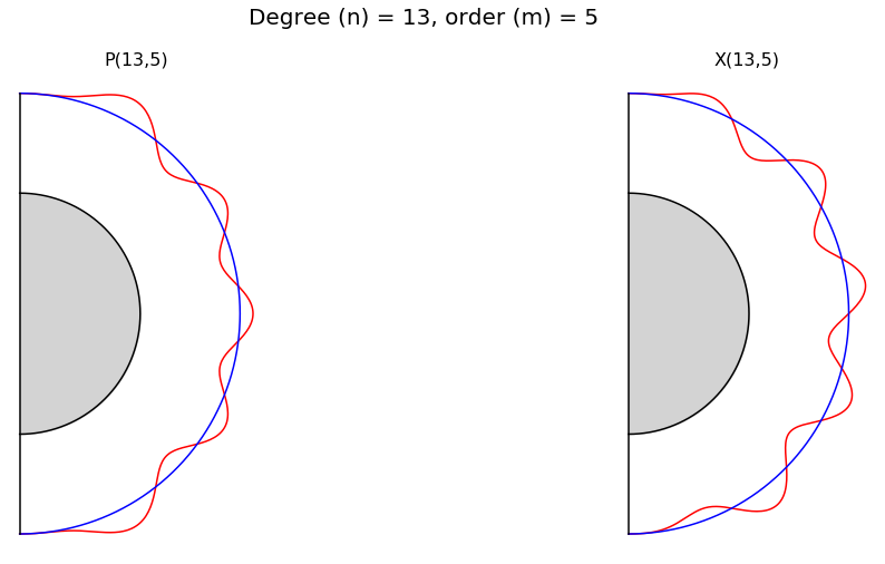
Plotting \(P_n^m\) and \(X_n^m\)
The \(P_n^m(\theta)\) and \(X_n^m(\theta)\) are building blocks for computing geomagnetic field models given a spherical harmonic model. It’s instructive to visualise these functions and below you can experiment by setting different values of spherical harmonic degree (\(n\)) and order (\(m \le n\)). Note how the choice of \(n\) and \(m\) affects the number of zeroes of the functions.
The functions are plotted on a semi-circle representing the surface of the Earth, with the inner core added for cosmetic purposes only! Again, purely for cosmetic purposes, the functions are scaled to fit within \(\pm\)10% of the Earth’s surface.
>> USER INPUT HERE: Set the spherical harmonic degree and order for the plot
degree = 13
order  = 5
# Calculate Pnm and Xmn values every 0.5 degrees
colat   = np.linspace(0,180,361)
pnmvals = np.zeros(len(colat))
xnmvals = np.zeros(len(colat))

idx     = sha.pnmindex(degree,order)
for i, cl in enumerate(colat):
    p,x = sha.pxyznm_calc(degree, cl)[0:2]
    pnmvals[i] = p[idx]
    xnmvals[i] = x[idx]

theta   = np.deg2rad(colat)
ct      = np.cos(theta)
st      = np.sin(theta)

# Numbers mimicking the Earth's surface and outer core radii
e_rad   = 6.371
c_rad   = 3.485

# Scale values to fit within 10% of "Earth's surface". Firstly the P(n,m),
shell   = 0.1*e_rad
pmax    = np.abs(pnmvals).max()
pnmvals = pnmvals*shell/pmax + e_rad
xp      = pnmvals*st
yp      = pnmvals*ct

# and now the X(n,m)
xmax    = np.abs(xnmvals).max()
xnmvals = xnmvals*shell/xmax + e_rad
xx      = xnmvals*st
yx      = xnmvals*ct

# Values to draw the Earth's and outer core surfaces as semi-circles
e_xvals = e_rad*st
e_yvals = e_rad*ct
c_xvals = e_xvals*c_rad/e_rad
c_yvals = e_yvals*c_rad/e_rad

# Earth-like background framework for plots
def eplot(ax):
    ax.set_aspect('equal')
    ax.set_axis_off()
    ax.plot(e_xvals,e_yvals, color='blue')
    ax.plot(c_xvals,c_yvals, color='black')
    ax.fill_between(c_xvals, c_yvals, y2=0, color='lightgrey')
    ax.plot((0, 0), (-e_rad, e_rad), color='black')

# Plot the P(n,m) and X(n,m)
fig, axes = plt.subplots(nrows=1, ncols=2, figsize=(18, 8))
fig.suptitle('Degree (n) = '+str(degree)+', order (m) = '+str(order), fontsize=20)

axes[0].plot(xp,yp, color='red')
axes[0].set_title('P('+ str(degree)+',' + str(order)+')', fontsize=16)
eplot(axes[0])

axes[1].plot(xx,yx, color='red')
axes[1].set_title('X('+ str(degree)+',' + str(order)+')', fontsize=16)
eplot(axes[1])
The International Geomagnetic Reference Field
The latest version of the IGRF is IGRF12 which consists of a main-field model every five years from 1900.0 to 2015.0 and a secular variation model for 2015-2020. The main field models have spherical harmonic degree (n) and order (m) 10 up to 1995 and n=m=13 from 2000 onwards. The secular variation model has n=m=8.
The coefficients are first loaded into a pandas database:
igrf12 = pd.read_csv(IGRF12_FILE, delim_whitespace=True,  header=3)
igrf12.head()  # Check the values have loaded correctly
| g/h | n | m | 1900.0 | 1905.0 | 1910.0 | 1915.0 | 1920.0 | 1925.0 | 1930.0 | ... | 1975.0 | 1980.0 | 1985.0 | 1990.0 | 1995.0 | 2000.0 | 2005.0 | 2010.0 | 2015.0 | 2015-20 | |
|---|---|---|---|---|---|---|---|---|---|---|---|---|---|---|---|---|---|---|---|---|---|
| 0 | g | 1 | 0 | -31543 | -31464 | -31354 | -31212 | -31060 | -30926 | -30805 | ... | -30100 | -29992 | -29873 | -29775 | -29692 | -29619.4 | -29554.63 | -29496.57 | -29442.0 | 10.3 |
| 1 | g | 1 | 1 | -2298 | -2298 | -2297 | -2306 | -2317 | -2318 | -2316 | ... | -2013 | -1956 | -1905 | -1848 | -1784 | -1728.2 | -1669.05 | -1586.42 | -1501.0 | 18.1 |
| 2 | h | 1 | 1 | 5922 | 5909 | 5898 | 5875 | 5845 | 5817 | 5808 | ... | 5675 | 5604 | 5500 | 5406 | 5306 | 5186.1 | 5077.99 | 4944.26 | 4797.1 | -26.6 |
| 3 | g | 2 | 0 | -677 | -728 | -769 | -802 | -839 | -893 | -951 | ... | -1902 | -1997 | -2072 | -2131 | -2200 | -2267.7 | -2337.24 | -2396.06 | -2445.1 | -8.7 |
| 4 | g | 2 | 1 | 2905 | 2928 | 2948 | 2956 | 2959 | 2969 | 2980 | ... | 3010 | 3027 | 3044 | 3059 | 3070 | 3068.4 | 3047.69 | 3026.34 | 3012.9 | -3.3 |
5 rows × 28 columns
a) Calculating geomagnetic field values using the IGRF
The function below calculates geomagnetic field values at a point defined by its colatitude, longitude and altitude, using a spherical harmonic model of maximum degree nmax supplied as an array gh. The parameter coord is a string specifying whether the input position is in geocentric coordinates (when altitude should be the geocentric distance in km) or geodetic coordinates (when altitude is distance above mean sea level in km).
It’s unconventional, but I’ve chosen to include a monopole term, set to zero, at index zero in the gh array.
def shm_calculator(gh, nmax, altitude, colat, long, coord):
    RREF     = 6371.2 #The reference radius assumed by the IGRF
    degree   = nmax
    phi      = long

    if (coord == 'Geodetic'):
        # Geodetic to geocentric conversion using the WGS84 spheroid
        rad, theta, sd, cd = sha.gd2gc(altitude, colat)
    else:
        rad   = altitude
        theta = colat

    # Function 'rad_powers' to create an array with values of (a/r)^(n+2) for n = 0,1, 2 ..., degree
    rpow = sha.rad_powers(degree, RREF, rad)

    # Function 'csmphi' to create arrays with cos(m*phi), sin(m*phi) for m = 0, 1, 2 ..., degree
    cmphi, smphi = sha.csmphi(degree,phi)

    # Function 'gh_phi_rad' to create arrays with terms such as [g(3,2)*cos(2*phi) + h(3,2)*sin(2*phi)]*(a/r)**5
    ghxz, ghy = sha.gh_phi_rad(gh, degree, cmphi, smphi, rpow)

    # Function 'pnm_calc' to calculate arrays of the Associated Legendre Polynomials for n (&m) = 0,1, 2 ..., degree
    pnm, xnm, ynm, znm = sha.pxyznm_calc(degree, theta)

    # Geomagnetic field components are calculated as a dot product
    X =  np.dot(ghxz, xnm)
    Y =  np.dot(ghy,  ynm)
    Z = -np.dot(ghxz, znm)

    # Convert back to geodetic (X, Y, Z) if required
    if (coord == 'Geodetic'):
        t = X
        X = X*cd + Z*sd
        Z = Z*cd - t*sd

    return((X, Y, Z))
>> >> USER INPUT HERE: Set the input parameters
location = 'Erehwon'
ctype    = 'Geodetic'  # coordinate type
altitude = 0           # in km above the spheroid if ctype = 'Geodetic', radial distance if ctype = 'Geocentric'
colat    = 35          # NB colatitude, not latitude
long     = -3          # longitude
NMAX     = 13          # Maxiimum spherical harmonic degree of the model
date     = 2015.0      # Date for the field estimates
Now calculate the IGRF geomagnetic field estimates.
# Calculate the gh values for the supplied date
if date == 2015.0:
    gh = igrf12['2015.0']
elif date < 2015.0:
    date_1 = (date//5)*5
    date_2 = date_1 + 5
    w1 = date-date_1
    w2 = date_2-date
    gh = np.array((w2*igrf12[str(date_1)] + w1*igrf12[str(date_2)])/(w1+w2))
elif date > 2015.0:
    gh =np.array(igrf12['2015.0'] + (date-2015.0)*igrf12['2015-20'])

gh = np.append(0., gh) # Add a zero monopole term corresponding to g(0,0)

bxyz = shm_calculator(gh, NMAX, altitude, colat, long, ctype)
dec, hoz ,inc , eff = mag.xyz2dhif(bxyz[0], bxyz[1], bxyz[2])

print('\nGeomagnetic field values at: ', location+', '+ str(date), '\n')
print('Declination (D):', '{: .1f}'.format(dec), 'degrees')
print('Inclination (I):', '{: .1f}'.format(inc), 'degrees')
print('Horizontal intensity (H):', '{: .1f}'.format(hoz), 'nT')
print('Total intensity (F)     :', '{: .1f}'.format(eff), 'nT')
print('North component (X)     :', '{: .1f}'.format(bxyz[0]), 'nT')
print('East component (Y)      :', '{: .1f}'.format(bxyz[1]), 'nT')
print('Vertical component (Z)  :', '{: .1f}'.format(bxyz[2]), 'nT')
Geomagnetic field values at:  Erehwon, 2015.0

Declination (D): -2.5 degrees
Inclination (I): -69.5 degrees
Horizontal intensity (H):  17399.1 nT
Total intensity (F)     :  49606.9 nT
North component (X)     :  17382.1 nT
East component (Y)      : -767.4 nT
Vertical component (Z)  : -46455.5 nT
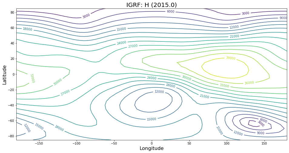
b) Maps of the IGRF
Now draw maps of the IGRF at the date selected above. The latitude range is set at -85 degrees to +85 degrees and the longitude range -180 degrees to +180 degrees and IGRF values for (X, Y, Z) are calculated on a 5 degree grid (this may take a few seconds to complete).
>> >> USER INPUT HERE: Set the element to plot
Enter the geomagnetic element to plot below:
D = declination
H = horizontal intensity
I = inclination
X = north component
Y = east component
Z = vertically (downwards) component
F = total intensity.)
el2plot = 'H'
def IGRF_plotter(el_name, vals, date):
    if el_name=='D':
        cvals = np.arange(-25,30,5)
    else:
        cvals = 15
    fig, ax = plt.subplots(figsize=(16, 8))
    cplt = ax.contour(longs, lats, vals, levels=cvals)
    ax.clabel(cplt, cplt.levels, inline=True, fmt='%d', fontsize=10)
    ax.set_title('IGRF: '+ el_name + ' (' + str(date) + ')', fontsize=20)
    ax.set_xlabel('Longitude', fontsize=16)
    ax.set_ylabel('Latitude', fontsize=16)
longs  = np.linspace(-180, 180, 73)
lats   = np.linspace(-85, 85, 35)
Bx, By, Bz = zip(*[sha.shm_calculator(gh,13,6371.2,90-lat,lon,'Geocentric') \
                 for lat in lats for lon in longs])
X = np.asarray(Bx).reshape(35,73)
Y = np.asarray(By).reshape(35,73)
Z = np.asarray(Bz).reshape(35,73)
D, H, I, F = [mag.xyz2dhif(X, Y, Z)[el] for el in range(4)]

el_dict={'X':X, 'Y':Y, 'Z':Z, 'D':D, 'H':H, 'I':I, 'F':F}
IGRF_plotter(el2plot, el_dict[el2plot], date)
Exercise
Produce a similar plot for the secular variation according to the IGRF.
References
Malin, S. R. . and Barraclough, D., (1981). An algorithm for synthesizing the geomagnetic field, Computers & Geosciences. Pergamon, 7(4), pp. 401–405. doi: 10.1016/0098-3004(81)90082-0.