.ipynb .pdf

repository open issue

JupyterHub

Contents

K Index Calculation

# Import notebook dependencies

import os
import sys
import numpy as np
import pandas as pd
import matplotlib.pyplot as plt
%matplotlib inline

sys.path.append('..')
from src import mag_lib as mag

# Set data paths
ESK_2003_PATH = os.path.abspath('../data/external/ESK_2003/')
K_INDS_PATH = os.path.abspath('../data/external/k_inds/')

Calculating K-indices for a single observatory

The K-index is a global geomagnetic activity index devised by Julius Bartels in 1938 to give a simple measure of the degree of geomagnetic disturbance during each 3-hour (UT) interval. It uses data from ground-based magnetometers to assign a number in the range 0-9 to interval, with K=0 indicating very little geomagnetic activity and K=9 representing an extreme geomagnetic storm. The K-index was introduced at the time of photographic recording, when magnetograms recorded variations in the horizontal geomagnetic field elements declination (D) and horizontal intensity (H), and in the vertical intensity (Z). To derive a K-index an observer would fit, by eye, a quiet-time curve to the records of D and H and measure the range (maximum-minimum) of the deviation of the recording from the curve. The K-index was then assigned according to a conversion table, with the greatest range in D and H ‘winning’. The north component (X) may be used instead of H, and the east component (Y) instead of D (X and Y will be used in the examples below). The vertical component Z is not used because it is liable to contamination by local induced currents.

The conversion from range in nanoteslas to index is quasi-logarithmic. The conversion table varies with latitude in an attempt to normalise the K-index distribution for observatories at different latitudes. The table for Eskdalemuir is shown below.

K	0	1	2	3	4	5	6	7	8	9
Lower bound (nT)	0	8	15	30	60	105	180	300	500	750

This means that, for instance, K=2 if the measured range is in the interval [15, 30] nT.

There was a VERY long debate in IAGA Division V about algorithms that could adequately reproduce the K-indices that an experienced observer would assign. The algorithms and code approved by IAGA are available at the International Service for Geomagnetic Indices: http://isgi.unistra.fr/softwares.php. (Also http://isgi.unistra.fr/what_are_kindices.php)

Example

In the following cells, we illustrate the process. A simple approach is to assume the so-called regular daily variation SR is made up of 24h, 12h and 8h signals (and, possibly, higher harmonics). A Fourier analysis can be used to investigate this. The functions in the cell below calculate Fourier coefficients from a data sample, and then synthesise a Fourier series using the coefficients.

Some days this simple approach seems to work well, on others it’s obviously wrong. Think about another approach you might take.

We will then attempt to calculate K-indices for the day selected by computing the Fourier series up the the number of harmonics selected by subtracting the synthetic harmonic signal from the data, then calculating 3-hr ranges and converting these into the corresponding K-index. The functions to do are also in the following cell.

def fourier(v, nhar):
    npts    = len(v)
    f       = 2.0/npts
    t       = np.linspace(0, npts, npts, endpoint=False)*2*np.pi/npts
    vmn     = np.mean(v)
    v       = v - vmn
    cofs    = [0]*(nhar+1)
    cofs[0] = (vmn,0)
    for i in range(1,nhar+1):
        c, s    = np.cos(i*t), np.sin(i*t)
        cofs[i] = (np.dot(v,c)*f, np.dot(v,s)*f)
    return (cofs)

def fourier_synth(cofs, npts):
    nt  = len(cofs)
    syn = np.zeros(npts)
    t  = np.linspace(0, npts, npts, endpoint=False)*2*np.pi/npts
    for n in range(1, nt):
        for j in range(npts):
            syn[j] += cofs[n][0]*np.cos(n*t[j]) + cofs[n][1]*np.sin(n*t[j])
    return (syn)

def K_plot(d, synd, day, E):
    fig, ax = plt.subplots(2, 1, figsize=(15, 10))
    t = np.linspace(0, 1440, 1440, endpoint= False)/60
    ax[0].plot(t, d)
    ax[0].plot(t, synd, color='red')
    ax[0].set_xlabel('UT (h)', fontsize=14)
    ax[0].set_ylabel(f'{E} (nT)', fontsize=14)
    ax[0].xaxis.set_ticks(np.arange(0, 27, 3))
    ax[0].set_title(f'K-index estimation: {OBSY} {day}, ({E}-range: {np.ptp(d):.1f}nT)', fontsize=20)
    ax[1].plot(t, d-synd)
    ax[1].set_xlabel('UT (h)', fontsize=14)
    ax[1].set_ylabel(f'{E} residuals (nT)', fontsize=14)
    ax[1].xaxis.set_ticks(np.arange(0, 27, 3))
    fig.tight_layout()

def K_calc(d, synd, Kb):
    tmp = np.ptp((d-synd).reshape(8,180), axis=1)
    return(list(np.digitize(tmp, bins=list(Kb.values()), right=False)-1))

def K_load(obscode, year, k_inds_path=K_INDS_PATH):
    kfile  = year + '.' + obscode
    filepath = os.path.join(k_inds_path, obscode, kfile)
    df = pd.read_csv(filepath, skiprows=0, header=None, delim_whitespace=True,  
                     parse_dates=[[2,1,0]], index_col=0)
    df = df.drop(3, axis=1)
    df.index.name='Date'
    return(df)

First, load in (X, Y, Z) one-minute data from Eskdalemuir for 2003 into a pandas dataframe.

OBSY = 'ESK'
year ='2003'
npts = 1440 # Number of minutes in a day
df = mag.load_year('esk', 2003, ESK_2003_PATH)
df.columns = [col.strip(OBSY) for col in df.columns]
df = df.drop(['DOY', 'F'], axis=1)
ann_means = df[[f'{i}' for i in 'XYZ']].resample('1Y').mean()
df.head()

	X	Y	Z
DATE_TIME
2003-01-01 00:00:00	17342.0	-1473.2	46197.8
2003-01-01 00:01:00	17341.5	-1473.4	46197.8
2003-01-01 00:02:00	17342.0	-1473.4	46197.8
2003-01-01 00:03:00	17342.2	-1473.8	46197.6
2003-01-01 00:04:00	17342.6	-1473.7	46197.6

>> USER INPUT HERE: Choose a day (2003-mm-dd) and the number of harmonics to calculate

Return here to investigate different days (note that only the file for 2003 is included in the data directory for this example).

day  = '2003-01-01'
nhar = 3

First convert the D variations to units of nT using the annual mean value of H. Then calculate the daily means of D and H.

xmn  = df[day].X.mean()
ymn  = df[day].Y.mean()
xmn, ymn

(17340.055069444443, -1477.117638888889)

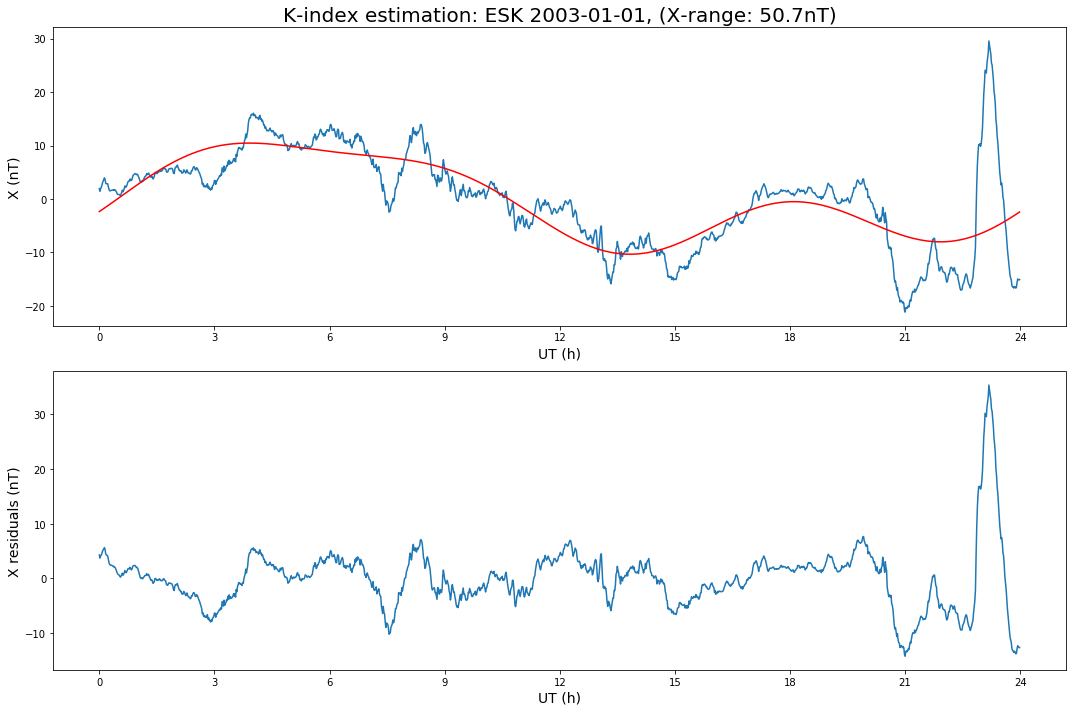
Now analyse the X data.

x     = df[day].X.values - xmn
xcofs = fourier(x, nhar)
synx  = fourier_synth(xcofs, npts)
K_plot(x, synx, day, 'X')

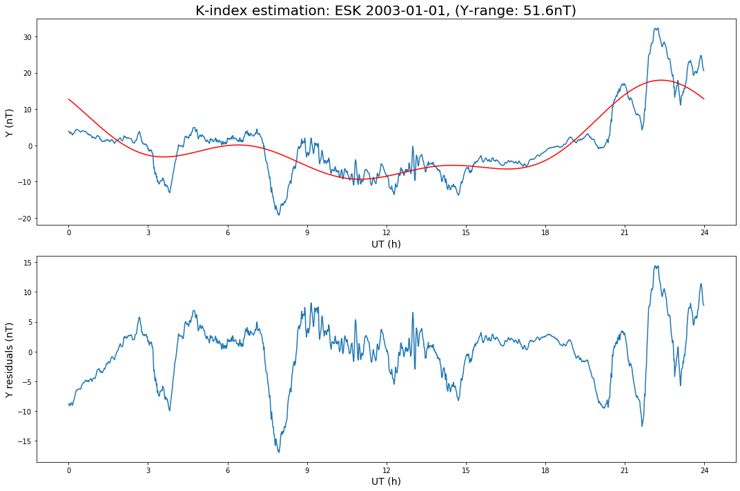
Repeat for Y.

y     = df[day].Y.values - ymn
ycofs = fourier(y, nhar)
syny  = fourier_synth(ycofs, npts)
K_plot(y, syny, day, 'Y')

Calculate the K-indices individually for the X and Y data, and also the final K index (the largest of the X and Y indices).

K_lb   = [0, 8, 15, 30, 60, 105, 180, 300, 500, 750]
K_dict = dict(zip([f'{OBSY}_K{i}' for i in range (10)], K_lb))
Kx = K_calc(x, synx, K_dict)
Ky = K_calc(y, syny, K_dict)
Kf =[max(Kx[i], Ky[i]) for i in range(8)]

Load the official 2003 observatory values for comparison and display the first few days.

dfk   = K_load(OBSY.lower(), year)
dfk.columns = ['00','03','06','09','12','15','18','21']
K_obs = list(dfk.loc[day])
dfk.head()

	00	03	06	09	12	15	18	21
Date
2003-01-01	1	2	2	1	1	1	2	3
2003-01-02	2	0	0	1	1	1	2	2
2003-01-03	2	0	1	1	3	5	4	4
2003-01-04	4	4	2	2	2	2	3	3
2003-01-05	1	1	1	1	2	2	2	3

Create a data frame containing all K values and print them out to compare.

K = pd.DataFrame({'K_x': Kx, 'K_y': Ky, 'K_final': Kf, 'K_obs': K_obs}).transpose()
K.columns = ['0','3','6','9','12','15','18','21']

print("Comparison of our K-indices with the official values")
K

Comparison of our K-indices with the official values

	0	3	6	9	12	15	18	21
K_x	1	1	2	1	1	1	2	3
K_y	1	2	2	1	1	0	1	2
K_final	1	2	2	1	1	1	2	3
K_obs	1	2	2	1	1	1	2	3

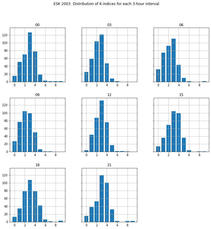
Plot histograms of the observed K-indices for each 3-hour period during 2003 in separate subplots

dfk.hist(figsize=(12,12), bins=[i for i in range(11)], sharey=True, align='left', rwidth=0.8)
plt.suptitle('ESK 2003: Distribution of K-indices for each 3-hour interval')

Text(0.5, 0.98, 'ESK 2003: Distribution of K-indices for each 3-hour interval')

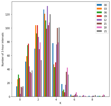
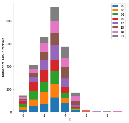
plotted side by side

plt.figure(figsize=(7,7))
plt.hist(dfk.values, bins=[i for i in range(11)], align='left')
plt.legend(dfk.columns)
plt.ylabel('Number of 3-hour intervals')
plt.xlabel('K')

Text(0.5, 0, 'K')

and stacked to give the distribution for the whole year

plt.figure(figsize=(7,7))
plt.hist(dfk.values, bins=[i for i in range(11)], stacked=True, align='left', rwidth=0.8)
plt.legend(dfk.columns)
plt.ylabel('Number of 3-hour intervals')
plt.xlabel('K')

Text(0.5, 0, 'K')

We also compute a daily sum of the K-indices for the 2003 file, and list days with high and low summed values. Note that this summation is not really appropriate because the K-index is quasi-logarithmic, however, this is a common simple measure of quiet and disturbed days. (These might be interesting days for you to look at.)

dfk['Ksum'] = dfk.sum(axis=1)
Ksort = dfk.sort_values('Ksum')
print('Quiet days: \n\n', Ksort.head(10), '\n\n')
print('Disturbed days: \n\n', Ksort.tail(10))

Quiet days: 

             00  03  06  09  12  15  18  21  Ksum
Date                                            
2003-10-11   1   0   0   0   1   0   0   0     2
2003-12-19   0   0   0   0   1   0   0   1     2
2003-12-18   1   1   0   0   1   0   0   0     3
2003-03-25   0   1   1   0   1   1   1   0     5
2003-12-25   1   0   0   0   2   1   0   1     5
2003-01-08   2   0   1   0   1   0   1   0     5
2003-01-09   0   0   0   0   0   1   2   2     5
2003-07-08   0   0   0   0   2   2   1   0     5
2003-10-12   0   0   0   1   1   0   2   2     6
2003-01-16   1   0   0   1   2   0   1   1     6 


Disturbed days: 

             00  03  06  09  12  15  18  21  Ksum
Date                                            
2003-09-17   4   5   4   4   5   5   4   5    36
2003-11-11   5   4   5   4   4   5   5   4    36
2003-02-02   5   4   4   4   4   6   5   5    37
2003-05-30   7   5   3   3   4   6   5   5    38
2003-05-29   3   3   3   2   6   6   7   8    38
2003-08-18   5   5   5   5   6   6   6   5    43
2003-11-20   1   3   5   4   7   9   9   8    46
2003-10-31   9   6   5   6   7   5   4   4    46
2003-10-30   8   5   4   4   5   5   9   9    49
2003-10-29   4   3   9   7   8   8   9   9    57

Note on the Fast Fourier Transform

In the examples above we computed Fourier coefficients in the ‘traditional’ way, so that if F(t) is a Fourier series representation of f(t), then,

F(t)=Ao+N∑n=1Ancos(2πntT)+Bnsin(2πntT)

where T is the fundamental period of F(t). The An and Bn are estimated by

Ao=1T∫T0f(t)dtAn=2T∫T0f(t)cos(2πntT)dtBn=2T∫T0f(t)sin(2πntT)dt

With N samples of digital data, the integral for An may be replaced by the summation

An=2TN−1∑j=0fjcos(2πnjΔtT)Δt=2NN−1∑j=0fjcos(2πnjN)

where the sampling interval Δt is given by T=NΔt and fj=f(jΔt). A similar expression applies for the Bn, and these are the coefficients returned by the function fourier above.

The fast Fourier transform (FFT) offers a computationally efficient means of finding the Fourier coefficients. The conventions for the FFT and its inverse (IFFT) vary from package to package. In the scipy.fftpack package, the FFT of a sequence xn of length N is defined as

yk=N−1∑n=0xnexp(−2πiknN)=N−1∑n=0xn(cos(2πknN)−isin(2πknN))

with the inverse defined as,

xn=1NN−1∑k=0ykexp(2πiknN)

The scipy documentation is a little inconsistent here because it explains the order of the yn as being y1,y2,…yN/2−1 as corresponding to increasing positive frequency and yN/2,yN/2+1,…yN−1 as ordered by decreasing negative frequency, for N even. (See: https://docs.scipy.org/doc/scipy/reference/tutorial/fftpack.html.)

The interpretation is that if yk=ak+ibk then will have (for N even), yN−k=ak−ibk and so

ak=12Re(yk+yN−k)bk=12Im(yk−yN−k)

and so we expect the relationship to the digitised Fourier series coefficients returned by the function fourier defined above to be,

Ak=−1NRe(ak+aN−k)Bk=−1NIm(bk−bN−k)

from scipy.fftpack import fft

# Compute the fft of the x data
xfft = fft(x)

# Compare results for the 24-hour component
k    = 1
print('Fourier coefficients: \n', f'A1 = {xcofs[1][0]} \n', f'B1 = {xcofs[1][1]} \n')
print('scipy FFT outputs: \n', f'a1 = {np.real(xfft[k]+xfft[npts-k])/npts} \n', \
      f'b1 = {-np.imag(xfft[k]-xfft[npts-k])/npts} \n')

Fourier coefficients: 
 A1 = 1.9222474131097547 
 B1 = 7.835093862256126 

scipy FFT outputs: 
 a1 = 1.922247413109754 
 b1 = 7.835093862256124 

References

Menvielle, M. et al. (1995) ‘Computer production of K indices: review and comparison of methods’, Geophysical Journal International. Oxford University Press, 123(3), pp. 866–886. doi: 10.1111/j.1365-246X.1995.tb06895.x.

Visualising geomagnetic data: time series, Bartels plots and contour plots Tracing magnetic field lines